Normalized Cuts on Region Adjacency Graphs

In my last post I demonstrated how removing edges with high weights can leave us with a set of disconnected graphs, each of which represents a region in the image. The main drawback however was that the user had to supply a threshold. This value varied significantly depending on the context of the image. For a fully automated approach, we need an algorithm that can remove edges automatically.

The first thing that I can think of which does something useful in the above mention situation is the Minimum Cut Algorithm. It divides a graph into two parts, A and B such that the weight of the edges going from nodes in Set A to the nodes in Set B is minimum.

For the Minimum Cut algorithm to work, we need to define the weights of our Region Adjacency Graph (RAG) in such a way that similar regions have more weight. This way, removing lesser edges would leave us with the similar regions.

Getting Started

For all the examples below to work, you will need to pull from this Pull Request. The tests fail due to outdated NumPy and SciPy versions on Travis. I have also submitted a Pull Request to fix that. Just like the last post, I have a show_img function.

from skimage import graph, data, io, segmentation, color
from matplotlib import pyplot as plt
from skimage.measure import regionprops
from skimage import draw
import numpy as np

def show_img(img):

    width = img.shape[1]/75.0
    height = img.shape[0]*width/img.shape[1]
    f = plt.figure(figsize=(width, height))
    plt.imshow(img)

I have modified the display_edges function for this demo. It draws nodes in yellow. Edges with low edge weights are greener and edges with high edge weight are more red.

def display_edges(image, g):
    """Draw edges of a RAG on its image

    Returns a modified image with the edges drawn. Edges with high weight are
    drawn in red and edges with a low weight are drawn in green. Nodes are drawn
    in yellow.

    Parameters
    ----------
    image : ndarray
        The image to be drawn on.
    g : RAG
        The Region Adjacency Graph.
    threshold : float
        Only edges in `g` below `threshold` are drawn.

    Returns:
    out: ndarray
        Image with the edges drawn.
    """

    image = image.copy()
    max_weight = max([d['weight'] for x, y, d in g.edges_iter(data=True)])
    min_weight = min([d['weight'] for x, y, d in g.edges_iter(data=True)])

    for edge in g.edges_iter():
        n1, n2 = edge

        r1, c1 = map(int, rag.node[n1]['centroid'])
        r2, c2 = map(int, rag.node[n2]['centroid'])

        green = 0,1,0
        red = 1,0,0

        line  = draw.line(r1, c1, r2, c2)
        circle = draw.circle(r1,c1,2)
        norm_weight = ( g[n1][n2]['weight'] - min_weight ) / ( max_weight - min_weight )

        image[line] = norm_weight*red + (1 - norm_weight)*green
        image[circle] = 1,1,0

    return image

To see demonstrate the display_edges function, I will load an image, which just has two regions of black and white.

demo_image = io.imread('bw.png')
show_img(demo_image)

Let’s compute the pre-segmenetation using the SLIC method. In addition to that, we will also use regionprops to give us the centroid of each region to aid the display_edges function.

labels = segmentation.slic(demo_image, compactness=30, n_segments=100)
labels = labels + 1  # So that no labelled region is 0 and ignored by regionprops
regions = regionprops(labels)

We will use label2rgb to replace each region with its average color. Since the image is so monotonous, the difference is hardly noticeable.

<

pre>

label_rgb = color.label2rgb(labels, demo_image, kind='avg')
show_img(label_rgb)

We can use mark_boundaries to display region boundaries.

label_rgb = segmentation.mark_boundaries(label_rgb, labels, (0, 1, 1))
show_img(label_rgb)

As mentioned earlier we need to construct a graph with similar regions having more weights between them. For this we supply the "similarity" option to rag_mean_color.

rag = graph.rag_mean_color(demo_image, labels, mode="similarity")

for region in regions:
    rag.node[region['label']]['centroid'] = region['centroid']

label_rgb = display_edges(label_rgb, rag)
show_img(label_rgb)

If you notice above the black and white regions have red edges between them, i.e. they are very similar. However the edges between the black and white regions are green, indicating they are less similar.

Problems with the min cut

Consider the following graph

The minimum cut approach would partition the graph as {A, B, C, D} and {E}. It has a tendency to separate out small isolated regions of the graph. This is undesirable for image segmentation as this would separate out small, relatively disconnected regions of the image. A more reasonable partition would be {A, C} and {B, D, E}. To counter this aspect of the minimum cut, we used the Normalized Cut.

The Normalized Cut

It is defined as follows
Let be the set of all nodes and for be the edge weight between and

where

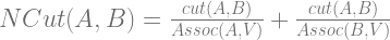
With the above equation, NCut won’t be low is any of A or B is not well-connected with the rest of the graph. Consider the same graph as the last one.

We can see that minimizing the NCut gives us the expected partition, that is, {A, C} and {B, D, E}.

Normalized Cuts for Image Segmentation

The idea of using Normalized Cut for segmenting images was first suggested by Jianbo Shi and Jitendra Malik in their paper Normalized Cuts and Image Segmentation. Instead of pixels, we are considering RAGs as nodes.

The problem of finding NCut is NP-Complete. Appendix A of the paper has a proof for it. It is made tractable by an approximation explained in Section 2.1 of the paper. The function _ncut_relabel is responsible for actually carrying out the NCut. It divides the graph into two parts, such that the NCut is minimized. Then for each of the two parts, it recursively carries out the same procedure until the NCut is unstable, i.e. it evaluates to a value greater than the specified threshold. Here is a small snippet to illustrate.

img = data.coffee()

labels1 = segmentation.slic(img, compactness=30, n_segments=400)
out1 = color.label2rgb(labels1, img, kind='avg')

g = graph.rag_mean_color(img, labels1, mode='similarity')
labels2 = graph.cut_normalized(labels1, g)
out2 = color.label2rgb(labels2, img, kind='avg')

show_img(out2)

NCut in Action

To observe how the NCut works, I wrote a small hack. This shows us the regions as divides by the method at every stage of recursion. The code relies on a modification in the original code, which can be seen here.

<

pre>

from skimage import graph, data, io, segmentation, color
from matplotlib import pyplot as plt
import os

#img = data.coffee()
os.system('rm *.png')
img = data.coffee()
#img = color.gray2rgb(img)

labels1 = segmentation.slic(img, compactness=30, n_segments=400)
out1 = color.label2rgb(labels1, img, kind='avg')

g = graph.rag_mean_color(img, labels1, mode='similarity')
labels2 = graph.cut_normalized(labels1, g)

offset = 1000
count = 1
tmp_labels = labels1.copy()
for g1,g2 in graph.graph_cut.sub_graph_list:
    for n,d in g1.nodes_iter(data=True):
        for l in d['labels']:
            tmp_labels[labels1 == l] = offset
    offset += 1
    for n,d in g2.nodes_iter(data=True):
        for l in d['labels']:
            tmp_labels[labels1 == l] = offset
    offset += 1
    tmp_img = color.label2rgb(tmp_labels, img, kind='avg')
    io.imsave(str(count) + '.png',tmp_img)
    count += 1

The two components at each stage are stored in the form of tuples in sub_graph_list. Let’s say, the Graph was divided into A and B initially, and later A was divided into A1 and A2. The first iteration of the loop will label A and B. The second iteration will label A1, A2 and B, and so on. I used the PNGs saved and converted them into a video with avconv using the command avconv -f image2 -r 1 -i %d.png -r 20 demo.webm. GIFs would result in a loss of color, so I made webm videos. Below are a few images and their respective successive NCuts. Use Full Screen for better viewing.

Note that although there is a user supplied threshold, it does not have to vary significantly. For all the demos below, the default value is used.

Colors Image

During each iteration, one region (area of the image with the same color) is split into two. A region is represented by its average color. Here’s what happens in the video

• The image is divided into red, and the rest of the regions (gray at this point)
• The grey is divided into a dark pink region (pink, maroon and yellow) and a
  dark green ( cyan, green and blue region ).
• The dark green region is divided into light blue ( cyan and blue ) and the
  green region.
• The light blue region is divided into cyan and blue
• The dark pink region is divided into yellow and a darker pink (pink and marron
  region.
• The darker pink region is divided into pink and maroon regions.

Coins Image

Camera Image

Coffee Image

Fruits Image

Baby Image ( Scaled )

Car Image

• computer vision
• gsoc
• image processing
• image-segmentation
• python
• RAG
• scikit-image