GSoC – Mid Term Status Update

So far

For the story so far see –  the Introduction, 2nd week update, Graph Data Structures Comparison .

After much debate on the mailing list with many scikit-image developers we finally decided to use the NetworkX Graph Class for our Region Adjacency Graph ( RAG ). It comes with a lot of well-tested functionality and would speed up the GSoC progress. It is also pure Python, and shares a lot of its dependencies with scikit-image.

Constructing the RAG

To construct a RAG, we need to iterate over the entire labeled image, looking for adjacent pixels with distinct labels. Initially I wrote a special case Cython loop for 2D and 3D, much like this one. But to scikit-image developers suggested, and rightly so, a more genaral n-dimensional approach. I looked for a function, which would iterate over an entire array and call a given function. As it turns out generic_filter does exactly that. I have used it here  with the callable defined here.

The footprint is created such that only the elements which are 2nd and 3rd along all axes are set according to the connectivity. Rest all are forced to zero. In the 2D case with connectivity 2 it would be the bottom right elements ( a[1,1], a[1,2] , a[2,1], a[2,2] ) which are set . This ensures that one pair of adjacent pixels is not processed again when the filter window moves ahead.

The footprint ensures that the first element in the array passed to the callable is the central element in the footprint. All other elements are adjacent to the central element and an edge is created between them and the central element.

Pruning the RAG

I implemented a skeletal RAG algorithm following Juan’s suggestion. It takes the labeled image as input. This is typically an over-segmented image obtained by algorithms like SLIC or watershed. Each region in the labeled image is represented by a node in the graph. Nodes of adjacent regions are joined by an edge. The weight of this edge is the magnitude of difference in mean color. Once the graph is constructed, nodes joined by edges with weights lesser than a given threshold are combined into one region.

You can view the Pull Request here.

Results

Below are the test results of executing the example code on two scikit-image sample images. The threshold value for both the results is different and is found by trial and error. Typically, a higher threshold value, gives fewer regions in the final image.

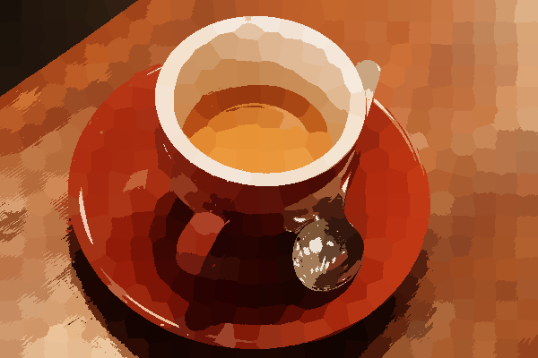
Coffee Image

Original Image

SLIC Segmentation

Threshold Graph Cut

 

Coins

Original Image

SLIC Segmentation

Threshold Graph Cut

Conclusion

The mechanism for RAGs is in place now. The segmentation is pretty satisfactory, considering the simple logic. The major drawback however is that it’s not fully automatic. Over the next few weeks I will implement more sophisticated merging predicates, including N-cut.

• gsoc
• image processing
• python